Density Estimation
Univariate Density Estimation
Parametric Desity Estimation
Draw from a normal distribution
Given \({{X}_{1}},{{X}_{2}},\ldots ,{{X}_{n}}\) \(i.i.d\) draw from a normal distribution with mean of \(\mu\) and variance of \({{\sigma }^{2}}\) the joint \(PDF\) can be expressed as: \[f\left( {{X}_{1}},{{X}_{2}},\ldots {{X}_{3}} \right)=\prod\limits_{i=1}^{n}{\frac{1}{\sqrt{2\pi {{\sigma }^{2}}}}{{e}^{-\frac{{{\left( {{X}_{i}}-\mu \right)}^{2}}}{2{{\sigma }^{2}}}}}}\] \[f\left( {{X}_{1}},{{X}_{2}},\ldots {{X}_{3}} \right)=\frac{1}{\sqrt{2\pi {{\sigma }^{2}}}}{{e}^{-\frac{{{\left( {{X}_{1}}-\mu \right)}^{2}}}{2{{\sigma }^{2}}}}}\times \frac{1}{\sqrt{2\pi {{\sigma }^{2}}}}{{e}^{-\frac{{{\left( {{X}_{2}}-\mu \right)}^{2}}}{2{{\sigma }^{2}}}}}\times \cdots \times \frac{1}{\sqrt{2\pi {{\sigma }^{2}}}}{{e}^{-\frac{{{\left( {{X}_{n}}-\mu \right)}^{2}}}{2{{\sigma }^{2}}}}}\] The term \(\frac{1}{\sqrt{2\pi {{\sigma }^{2}}}}\) is a constant multiplying this term for \(n\) times gives \({{\left( \frac{1}{\sqrt{2\pi {{\sigma }^{2}}}} \right)}^{n}}=\frac{1}{{{\left( 2\pi \sigma \right)}^{\frac{n}{2}}}}\). \[f\left( {{X}_{1}},{{X}_{2}},\ldots {{X}_{3}} \right)=\frac{1}{{{\left( 2\pi \sigma \right)}^{\frac{n}{2}}}}{{e}^{-\frac{{{\left( {{X}_{1}}-\mu \right)}^{2}}}{2{{\sigma }^{2}}}}}\times {{e}^{-\frac{{{\left( {{X}_{2}}-\mu \right)}^{2}}}{2{{\sigma }^{2}}}}}\times \cdots \times {{e}^{-\frac{{{\left( {{X}_{n}}-\mu \right)}^{2}}}{2{{\sigma }^{2}}}}}\] With the index law of addition i.e. we can add the indices for the same base \[{{e}^{-\frac{{{\left( {{X}_{1}}-\mu \right)}^{2}}}{2{{\sigma }^{2}}}}}\times {{e}^{-\frac{{{\left( {{X}_{2}}-\mu \right)}^{2}}}{2{{\sigma }^{2}}}}}\times \cdots \times {{e}^{-\frac{{{\left( {{X}_{n}}-\mu \right)}^{2}}}{2{{\sigma }^{2}}}}}={{e}^{-\frac{1}{2{{\sigma }^{2}}}\left\{ {{\left( {{X}_{1}}-\mu \right)}^{2}}+{{\left( {{X}_{2}}-\mu \right)}^{2}}+\cdots +{{\left( {{X}_{n}}-\mu \right)}^{2}} \right\}}}={{e}^{-\frac{1}{2{{\sigma }^{2}}}\sum\limits_{i=1}^{n}{{{\left( Xi-\mu \right)}^{2}}}}}\] Therefore, \[f\left( {{X}_{1}},{{X}_{2}},\ldots {{X}_{3}} \right)=\frac{1}{{{\left( 2\pi {{\sigma }^{2}} \right)}^{\frac{n}{2}}}}{{e}^{-\frac{1}{2{{\sigma }^{2}}}\sum\nolimits_{i=1}^{n}{{{\left( {{X}_{i}}-\mu \right)}^{2}}}}}\]
The log-likelihood function
Taking the logarithm, we get the log-likelihood function as: \[\ln f\left( {{X}_{1}},{{X}_{2}},\ldots {{X}_{3}} \right)=\ln \left[ \frac{1}{{{\left( 2\pi {{\sigma }^{2}} \right)}^{\frac{n}{2}}}}{{e}^{-\frac{1}{2{{\sigma }^{2}}}\sum\nolimits_{i=1}^{n}{{{\left( {{X}_{i}}-\mu \right)}^{2}}}}} \right]\]
With the property of log i.e. multiplication inside the log can be turned into addition outside the log, and vice versa or \(\ln (ab)=\ln (a)+\ln (b)\) \[L\left( \mu ,{{\sigma }^{2}} \right)\equiv \ln \left( \frac{1}{{{\left( 2\pi {{\sigma }^{2}} \right)}^{\frac{n}{2}}}} \right)+\ln \left( {{e}^{-\frac{1}{2{{\sigma }^{2}}}\sum\nolimits_{i=1}^{n}{{{\left( {{X}_{i}}-\mu \right)}^{2}}}}} \right)\] With natural log property i.e. when \({{e}^{y}}=x\) then \(\ln (x)=\ln ({{e}^{y}})=y\) \[L\left( \mu ,{{\sigma }^{2}} \right)\equiv \ln \left( {{\left( 2\pi {{\sigma }^{2}} \right)}^{-\frac{n}{2}}} \right)-\frac{1}{2{{\sigma }^{2}}}\sum\nolimits_{i=1}^{n}{{{\left( {{X}_{i}}-\mu \right)}^{2}}}\] \[L\left( \mu ,{{\sigma }^{2}} \right)\equiv -\frac{n}{2}\ln \left( 2\pi \right)-\frac{n}{2}\ln {{\sigma }^{2}}-\frac{1}{2{{\sigma }^{2}}}\sum\nolimits_{i=1}^{n}{{{\left( {{X}_{i}}-\mu \right)}^{2}}}\] \[L\left( \mu ,{{\sigma }^{2}} \right)\equiv \ln f\left( {{X}_{1}},{{X}_{2}},\ldots ,{{X}_{n}};\mu ,{{\sigma }^{2}} \right)=-\frac{n}{2}\ln \left( 2\pi \right)-\frac{n}{2}\ln \left( {{\sigma }^{2}} \right)-\frac{1}{2{{\sigma }^{2}}}\sum\nolimits_{i=1}^{n}{{{\left( {{X}_{i}}-\mu \right)}^{2}}}\]
Logliklihood function optimization
To find the optimum value of \(L\left( \mu ,{{\sigma }^{2}} \right)\equiv \ln f\left( {{X}_{1}},{{X}_{2}},\ldots ,{{X}_{n}};\mu ,{{\sigma }^{2}} \right)=-\frac{n}{2}\ln \left( 2\pi \right)-\frac{n}{2}\ln \left( {{\sigma }^{2}} \right)-\frac{1}{2{{\sigma }^{2}}}\sum\nolimits_{i=1}^{n}{{{\left( {{X}_{i}}-\mu \right)}^{2}}}\), we take the first order condition w.r.t. \(\mu\) and \({{\sigma }^{2}}\). The necessary first order condition w.r.t \(\mu\) is given as: \[\frac{\partial L\left( \mu ,{{\sigma }^{2}} \right)}{\partial \mu }=\frac{\partial }{\partial \mu }\left\{ -\frac{n}{2}\ln \left( 2\pi \right)-\frac{n}{2}\ln \left( {{\sigma }^{2}} \right)-\frac{1}{2{{\sigma }^{2}}}\sum\nolimits_{i=1}^{n}{{{\left( {{X}_{i}}-\mu \right)}^{2}}} \right\}=0\] Here, \(\frac{\partial }{\partial \mu }\left\{ -\frac{n}{2}\ln \left( 2\pi \right) \right\}=0\) and \(\frac{\partial }{\partial \mu }\left\{ -\frac{n}{2}\ln \left( {{\sigma }^{2}} \right) \right\}=0\), so we only need to solve for \[\frac{\partial }{\partial \mu }\left\{ -\frac{1}{2{{\sigma }^{2}}}\sum\nolimits_{i=1}^{n}{{{\left( {{X}_{i}}-\mu \right)}^{2}}} \right\}=0\] \[-\frac{1}{2{{\sigma }^{2}}}\frac{\partial }{\partial \mu }\sum\nolimits_{i=1}^{n}{{{\left( {{X}_{i}}-\mu \right)}^{2}}}=0\] \[-\frac{1}{2{{\sigma }^{2}}}\left[ \frac{\partial }{\partial \mu }\left\{ {{\left( {{X}_{1}}-\mu \right)}^{2}}+{{\left( {{X}_{2}}-\mu \right)}^{2}}+\cdots +{{\left( {{X}_{n}}-\mu \right)}^{2}} \right\} \right]=0\] \[-\frac{1}{2{{\sigma }^{2}}}\left[ \frac{\partial {{\left( {{X}_{1}}-\mu \right)}^{2}}}{\partial \mu }+\frac{\partial {{\left( {{X}_{2}}-\mu \right)}^{2}}}{\partial \mu }+\cdots +\frac{\partial {{\left( {{X}_{n}}-\mu \right)}^{2}}}{\partial \mu } \right]=0\] With the chain rule i.e \(\frac{\partial {{\left( {{X}_{1}}-\mu \right)}^{2}}}{\partial \mu }=\frac{\partial {{\left( {{X}_{1}}-\mu \right)}^{2}}}{\partial \left( {{X}_{1}}-\mu \right)}\frac{\partial \left( {{X}_{1}}-\mu \right)}{\partial \mu }=2\left( {{X}_{1}}-\mu \right)\left( 1 \right)=2\left( {{X}_{1}}-\mu \right)\). Hence, \[-\frac{1}{2{{\sigma }^{2}}}\left[ 2\left( {{X}_{1}}-\mu \right)+2\left( {{X}_{2}}-\mu \right)+\cdots +2\left( {{X}_{n}}-\mu \right) \right]=0\] \[-\frac{1}{{{\sigma }^{2}}}\sum\limits_{i=1}^{n}{\left( {{X}_{i}}-\mu \right)}=0\] Since \({{\sigma }^{2}}\ne 0\), So, \[\sum\limits_{i=1}^{n}{\left( {{X}_{i}}-\mu \right)}=0\] \[\sum\limits_{i=1}^{n}{{{X}_{i}}}-\sum\limits_{i=1}^{n}{\mu }=0\] \[\sum\limits_{i=1}^{n}{{{X}_{i}}}-n\mu =0\] \[\hat{\mu }={{n}^{-1}}\sum\limits_{i=1}^{n}{{{X}_{i}}}\]
The necessary first order condition w.r.t \({{\sigma }^{2}}\) is given as:
\[\frac{\partial L\left( \mu ,{{\sigma }^{2}} \right)}{\partial {{\sigma }^{2}}}=\frac{\partial }{\partial {{\sigma }^{2}}}\left\{ -\frac{n}{2}\ln \left( 2\pi \right)-\frac{n}{2}\ln \left( {{\sigma }^{2}} \right)-\frac{1}{2{{\sigma }^{2}}}\sum\nolimits_{i=1}^{n}{{{\left( {{X}_{i}}-\mu \right)}^{2}}} \right\}=0\]
\[-\frac{\partial }{\partial {{\sigma }^{2}}}\left\{ \frac{n}{2}\ln \left( 2\pi \right) \right\}-\frac{\partial }{\partial {{\sigma }^{2}}}\left\{ -\frac{n}{2}\ln \left( {{\sigma }^{2}} \right) \right\}-\frac{\partial }{\partial {{\sigma }^{2}}}\left\{ \frac{1}{2{{\sigma }^{2}}}\sum\nolimits_{i=1}^{n}{{{\left( {{X}_{i}}-\mu \right)}^{2}}} \right\}=0\]
\[0-\frac{n}{2}\frac{1}{{{\sigma }^{2}}}-\frac{1}{2}\sum\nolimits_{i=1}^{n}{{{\left( {{X}_{i}}-\mu \right)}^{2}}}\frac{\partial {{\left( {{\sigma }^{2}} \right)}^{-1}}}{\partial {{\sigma }^{2}}}=0\]
\[-\frac{1}{2}\sum\nolimits_{i=1}^{n}{{{\left( {{X}_{i}}-\mu \right)}^{2}}}\left( -1 \right){{\left( {{\sigma }^{2}} \right)}^{-2}}=\frac{n}{2{{\sigma }^{2}}}\]
\[\frac{1}{2{{\left( {{\sigma }^{2}} \right)}^{2}}}\sum\nolimits_{i=1}^{n}{{{\left( {{X}_{i}}-\mu \right)}^{2}}}=\frac{n}{2{{\sigma }^{2}}}\]
\[{{\hat{\sigma }}^{2}}={{n}^{-1}}\sum\nolimits_{i=1}^{n}{{{\left( {{X}_{i}}-\mu \right)}^{2}}}\]
\(\hat{\mu }\) and \({{\hat{\sigma }}^{2}}\) above are the maximum likelihood estimator of \(\mu\) and \({{\sigma }^{2}}\), respectively, the resulting estimator of \(f\left( x \right)\) is: \[\hat{f}\left( x \right)=\frac{1}{\sqrt{2\pi {{{\hat{\sigma }}}^{2}}}}{{e}^{\left[ -\frac{1}{2}\left( \frac{x-\hat{\mu }}{{{{\hat{\sigma }}}^{2}}} \right) \right]}}\]
Simulation example
Let’s simulate 10000 random observation from a normal distribution with mean of 2 and standard deviation of 1.5. To reproduce the results we will use set.seed() function.
set.seed(1234)
N <- 10000
mu <- 2
sigma <- 1.5
x <- rnorm(n = N, mean = mu, sd = sigma)
We can use mean() and sd() function to find the mean and sigma
# mean
sum(x)/length(x)
## [1] 2.009174mean(x)## [1] 2.009174# standard deviation
sqrt(sum((x-mean(x))^2)/(length(x)-1))## [1] 1.481294sd(x)## [1] 1.481294However, if can also simulate and try the optimization using the mle function from the stat 4 package in R.
LL <- function(mu, sigma){
  R <- dnorm(x, mu, sigma)
  -sum(log(R))
}

stats4::mle(LL, start = list(mu = 1, sigma = 1))
##
## Call:
## stats4::mle(minuslogl = LL, start = list(mu = 1, sigma = 1))
##
## Coefficients:
## mu sigma
## 2.009338 1.481157To supress the warnings in R and garanatee the solution we can use following codes.
stats4::mle(LL, start = list(mu = 1, sigma = 1), method = "L-BFGS-B",
            lower = c(-Inf, 0), upper = c(Inf, Inf))
##
## Call:
## stats4::mle(minuslogl = LL, start = list(mu = 1, sigma = 1),
## method = "L-BFGS-B", lower = c(-Inf, 0), upper = c(Inf, Inf))
##
## Coefficients:
## mu sigma
## 2.009174 1.481221Density plot example
Given the data of x = (-0.57, 0.25, -0.08, 1.40, -1.05, 1.00, 0.37, -1.15, 0.73, 1.59), we can estimate \(\hat{\mu }\) as sum(x)/length(x) or mean(x) and \({{\hat{\sigma }}^{2}}\) as sum((x-mean(x))^2)/(length(x)-1) or var(x). Note I use the sample variance formula.
x <- c(-0.57, 0.25, -0.08, 1.40, -1.05, 1.00, 0.37, -1.15, 0.73, 1.59)

# mean
sum(x)/length(x)
## [1] 0.249mean(x)## [1] 0.249# variance
sum((x-mean(x))^2)/(length(x)-1)## [1] 0.9285211var(x)## [1] 0.9285211We can also plot a parametric density function. But prior we plot, we have to sort the data.
x <- sort(x)
plot(x ,dnorm(x,mean=mean(x),sd=sd(x)),ylab="Density",type="l", col = "blue", lwd = 3)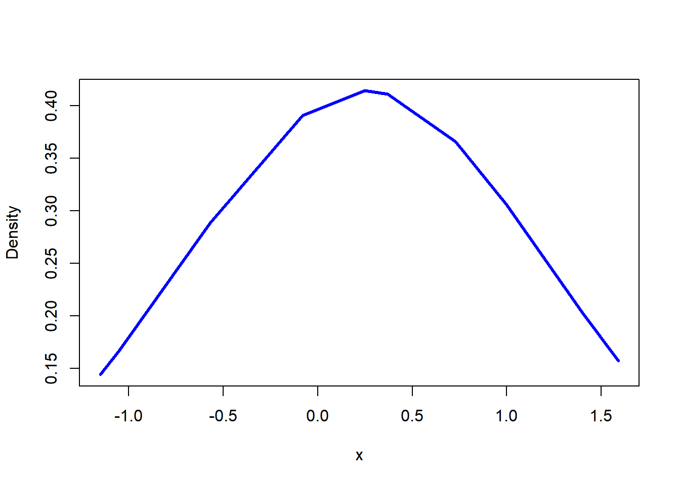
Let’s also plot a graph of histogram using bin width ranging from -1.5 through 2.0.
hist(x, breaks=seq(-1.5,2,by=0.5), prob = TRUE)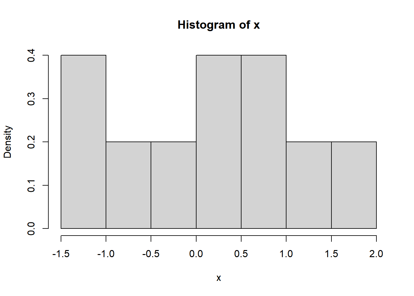
Univariate NonParametric Density Estimation
Set-up
Consider \(i.i.d\) data \({{X}_{1}},{{X}_{2}},\ldots ,{{X}_{n}}\) with \(F\left( \centerdot \right)\) an unknown \(CDF\) where \(F\left( x \right)=P\left[ X\le x \right]\) or \(CDF\) of \(X\) evaluated at \(x\). We can do a na?ve estimation as \(F\left( x \right)=P\left[ X\le x \right]\) as cumulative sums of relative frequency as:
\[{{F}_{n}}\left( x \right)={{n}^{-1}}\left\{ \#\ of\ {{X}_{i}}\le x \right\}\] and \(n\to\infty\) yields \({{F}_{n}}\left( x \right)\to F\left( x \right)\).
The \(PDF\) of \(F\left( x \right)=P\left[ X\le x \right]\) is given as \(f\left( x \right)=\frac{d}{dx}F\left( x \right)\) and an obvious estimator is: \[\hat{f}\left( x \right)=\frac{rise}{run}=\frac{{{F}_{n}}\left( x+h \right)-{{F}_{n}}\left( x-h \right)}{x+h-\left( x-h \right)}=\frac{{{F}_{n}}\left( x+h \right)-{{F}_{n}}\left( x-h \right)}{2h}={{n}^{-1}}\frac{1}{2h}\left\{ \#\ of\ {{X}_{i}}\ in\ between\ \left[ x-h,x+h \right] \right\}\]
Naive Kernel
The \(k\left( \centerdot \right)\) can be any kernel function, If we define a uniform kernel function or also known as na?ve kernel function then \[k\left( z \right)=\left\{ \begin{matrix} {1}/{2}\; & if\ \left| z \right|\le 1 \\ 0 & o.w \\ \end{matrix} \right.\] Where \(\left| {{z}_{i}} \right|=\left| \frac{{{X}_{i}}-x}{h} \right|\) and therefore is symmetric and hence \(\#\ of\ {{X}_{i}}\ in\ between\ \left[ x-h,x+h \right]\) means \(2\left( \frac{{{X}_{i}}-x}{h} \right)\). Then it is easy to see \(\hat{f}\left( x \right)\) to be expressed as: \[\hat{f}\left( x \right)=\frac{1}{2h}{{n}^{-1}}\left\{ \#\ of\ {{X}_{i}}\ in\ between\ \left[ x-h,x+h \right] \right\}=\frac{1}{2h}{{n}^{-1}}\sum\limits_{i=1}^{n}{k\left( 2\frac{{{X}_{i}}-x}{h} \right)}=\frac{1}{nh}\sum\limits_{i=1}^{n}{k\left( \frac{{{X}_{i}}-x}{h} \right)}\]
We can use follwoing code for naive kernel.
x <- c(-0.57, 0.25, -0.08, 1.40, -1.05, 1.00, 0.37, -1.15, 0.73, 1.59)
x <- sort(x)

naive_kernel <- function(x,y,h){
  z <- (x-y)/h
  ifelse(abs(z) <= 1, 1/2, 0)
}

naive_density <- function(x, h){
  val <- c()
  for(i in 1:length(x)) {
    val[i] <- sum(naive_kernel(x,x[i],h)/(length(x)*h))
  }
  val
}

H <- c(0.5, 1.0, 1.5)

names <- as.vector(paste0("H = ", H))
density_data <- list()
for(i in 1:length(H)){
  density_data[[i]] <- naive_density(x, H[i])
}
density_data <- do.call(cbind.data.frame, density_data)
colnames(density_data) <- names


matplot(density_data, type = "b", xlab = "x",
        ylab = "Density", pch=1:length(H), col = 1:length(H),
        main = "Naive Density for various Smoothing Parameter H")
legend("topleft", legend=names,  bty = "n", pch=1:length(H), col = 1:length(H))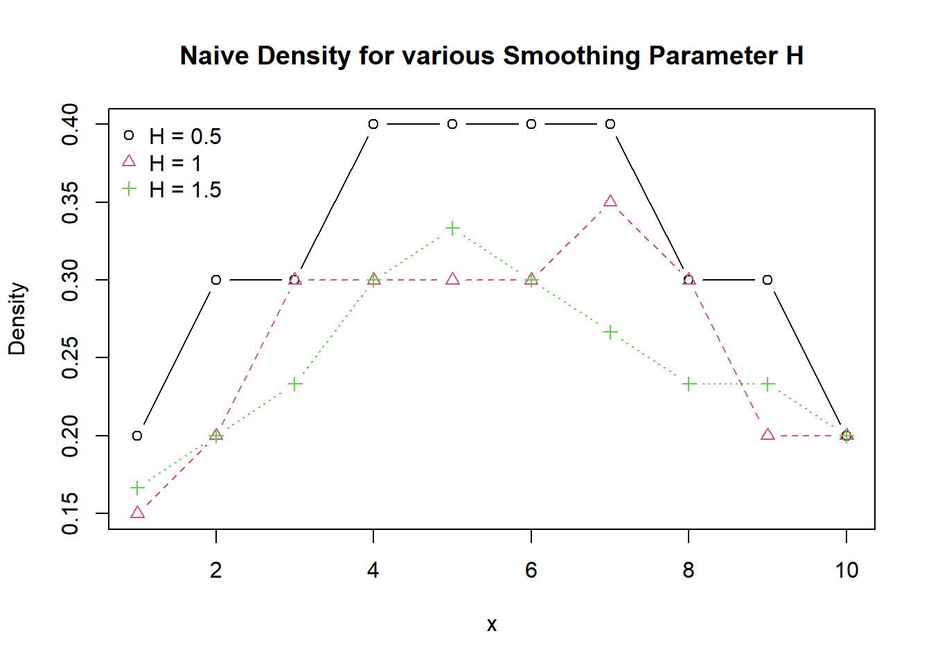
Epanechnikov kernel
Consider another optimal kernel known as Epanechnikov kernel given by: \[k\left( \frac{{{X}_{i}}-x}{h} \right)=\left\{ \begin{matrix} \frac{3}{4\sqrt{5}}\left( 1-\frac{1}{5}{{\left( \frac{{{X}_{i}}-x}{h} \right)}^{2}} \right) & if\ \left| \frac{{{X}_{i}}-x}{h} \right|<5 \\ 0 & o.w \\ \end{matrix} \right.\] Let’s use x = (-0.57, 0.25, -0.08, 1.40, -1.05, 1.00, 0.37, -1.15, 0.73, 1.59) and compute the kernel estimator of the density function of every sample realization using bandwidth of \(h=0.5\), \(h=1\), \(h=1.5\), where, \(h\) is smoothing parameter restricted to lie in the range of \((0,\infty ]\). We can use follwoing codes to estimate the density using Epanechnikov kernel.
x <- c(-0.57, 0.25, -0.08, 1.40, -1.05, 1.00, 0.37, -1.15, 0.73, 1.59)
x <- sort(x)

epanichnikov_kernel <- function(x,y,h){
  z <- (x-y)/h
  ifelse(abs(z) < sqrt(5), (1-z^2/5)*(3/(4*sqrt(5))), 0)
}

epanichnikov_density <- function(x, h){
  val <- c()
  for(i in 1:length(x)) {
    val[i] <- sum(epanichnikov_kernel(x,x[i],h)/(length(x)*h))
  }
  val
}

H <- c(0.5, 1.0, 1.5)

names <- as.vector(paste0("H = ", H))
density_data <- list()
for(i in 1:length(H)){
  density_data[[i]] <- epanichnikov_density(x, H[i])
}
density_data <- do.call(cbind.data.frame, density_data)
colnames(density_data) <- names


matplot(density_data, type = "b", xlab = "x",
        ylab = "Density", pch=1:length(H), col = 1:length(H),
        main = "Epanichnikov Density for various Smoothing Parameter H")
legend("topleft", legend=names,  bty = "n", pch=1:length(H), col = 1:length(H))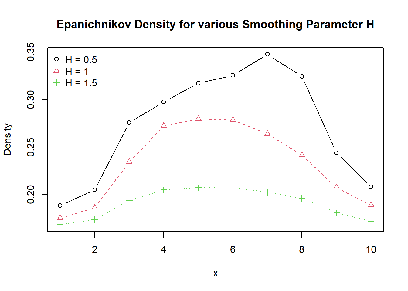
Three properties of kernel estimator
For any general nonnegative bounded kernel function \(k\left( v \right)\) where \(v=\left( \frac{{{X}_{i}}-x}{h} \right)\), the kernel estimator \(\hat{f}\left( x \right)\) is a consistent estimator of \(f\left( x \right)\) that satisfies three conditions: First is area under a kernel to be unity. \[\int{k(v)dv=1}\]
Second is the symmetry kernel \[\int{vk(v)dv=0}\] which implies symmetry condition i.e. \(k(v)=k(-v)\). For asymmetric kernels see Abadir and Lawford (2004).
Third is a positive constant. \[\int{{{v}^{2}}k(v)dv={{\kappa }_{2}}>0}\]
The big O and small o.
Taylor series expansion
For a univariate function \(g(x)\)evaluated at \({{x}_{0}}\) , we can express with Taylor series expansion as: \[g(x)=g({{x}_{0}})+{{g}^{(1)}}({{x}_{0}})(x-{{x}_{0}})+\frac{1}{2!}{{g}^{(2)}}({{x}_{0}}){{(x-{{x}_{0}})}^{2}}+\cdots +\frac{1}{(m-1)!}{{g}^{(m-1)}}({{x}_{0}}){{(x-{{x}_{0}})}^{m-1}}+\frac{1}{(m)!}{{g}^{(m)}}({{x}_{0}}){{(x-{{x}_{0}})}^{m}}+\cdots \] For a univariate function \(g(x)\)evaluated at \({{x}_{0}}\) that is \(m\) times differentiable, we can express with Taylor series expansion as: \[g(x)=g({{x}_{0}})+{{g}^{(1)}}({{x}_{0}})(x-{{x}_{0}})+\frac{1}{2!}{{g}^{(2)}}({{x}_{0}}){{(x-{{x}_{0}})}^{2}}+\cdots +\frac{1}{(m-1)!}{{g}^{(m-1)}}({{x}_{0}}){{(x-{{x}_{0}})}^{m-1}}+\frac{1}{(m)!}{{g}^{(m)}}(\xi ){{(x-{{x}_{0}})}^{m}}\] Wwhere \({{g}^{(s)}}={{\left. \frac{{{\partial }^{s}}g(x)}{\partial {{x}^{2}}} \right|}_{x={{x}_{0}}}}\) and and \(\xi\) lies between \(x\) and \({{x}_{0}}\)
MSE, variance and biases
Say \(\hat{\theta }\) is an estimator for true \(\theta\), then the Mean Squared Error \(MSE\) of an estimator \(\hat{\theta }\) is the mean of squared deviation between \(\hat{\theta }\) and \(\theta\) and given as: \[MSE=E\left[ {{\left( \hat{\theta }-\theta \right)}^{2}} \right] \] \[MSE=E\left[ \left( {{{\hat{\theta }}}^{2}}-2\hat{\theta }\theta +{{\theta }^{2}} \right) \right] \] \[MSE=E[{{\hat{\theta }}^{2}}]+E[{{\theta }^{2}}]-2\theta E[\hat{\theta }]\] \[MSE=\underbrace{E[{{{\hat{\theta }}}^{2}}]-{{E}^{2}}[{{{\hat{\theta }}}^{2}}]}_{\operatorname{var}(\hat{\theta })}+\underbrace{{{E}^{2}}[{{{\hat{\theta }}}^{2}}]+E[{{\theta }^{2}}]-2\theta E[\hat{\theta }]}_{E{{\left( E[\hat{\theta }]-\theta \right)}^{2}}}\] \[MSE=\operatorname{var}(\hat{\theta })+\underbrace{E{{\left( E[\hat{\theta }]-\theta \right)}^{2}}}_{squared\ of\ bias\ of\ \hat{\theta }}\] \[MSE=\operatorname{var}(\hat{\theta })+{{\left\{ bias(\hat{\theta }) \right\}}^{2}}\]
Note: \(\underbrace{E{{\left( \hat{\theta }-E[\hat{\theta }] \right)}^{2}}}_{\operatorname{var}(\hat{\theta })}=\underbrace{E[{{{\hat{\theta }}}^{2}}]-{{E}^{2}}[{{{\hat{\theta }}}^{2}}]}_{\operatorname{var}(\hat{\theta })}\).
Another way of solution is given as : \[MSE=E\left[ {{\left( \hat{\theta }-\theta \right)}^{2}} \right] \] \[MSE=E\left[ {{\left( \hat{\theta }-E[\hat{\theta }]+E[\hat{\theta }]-\theta \right)}^{2}} \right]\] \[MSE=E\left[ {{\left( \hat{\theta }-E[\hat{\theta }] \right)}^{2}}+{{\left( E[\hat{\theta }]-\theta \right)}^{2}}+2\left( \hat{\theta }-E[\hat{\theta }] \right)\left( E[\hat{\theta }]-\theta \right) \right]\] \[MSE=\underbrace{E{{\left( \hat{\theta }-E[\hat{\theta }] \right)}^{2}}}_{\operatorname{var}(\hat{\theta })}+\underbrace{E{{\left( E[\hat{\theta }]-\theta \right)}^{2}}}_{squared\ of\ bias\ of\hat{\theta }}+2E\left[ \left( \hat{\theta }-E[\hat{\theta }] \right)\left( E[\hat{\theta }]-\theta \right) \right]\] \[MSE=\operatorname{var}(\hat{\theta })+{{\left\{ bias(\hat{\theta }) \right\}}^{2}}+2E\left[ \left( \hat{\theta }E[\hat{\theta }]+\hat{\theta }\theta -E[\hat{\theta }]E[\hat{\theta }]-E[\hat{\theta }]\theta \right) \right]\] \[MSE=\operatorname{var}(\hat{\theta })+{{\left\{ bias(\hat{\theta }) \right\}}^{2}}+2E\left[ \left( \underbrace{\hat{\theta }E[\hat{\theta }]-E[\hat{\theta }]E[\hat{\theta }]}_{0}+\underbrace{\hat{\theta }\theta -E[\hat{\theta }]\theta }_{0} \right) \right]\] \[MSE=\operatorname{var}(\hat{\theta })+{{\left\{ bias(\hat{\theta }) \right\}}^{2}}\]
Theorem 1.1.
Let \({{X}_{1}},{{X}_{2}},\ldots ,{{X}_{n}}\) \(i.i.d\) observation having a three-times differentiable \(PDF\) \(f(x)\), and \({{f}^{s}}(x)\) denote the \(s-th\) order derivative of \(f(x)\ s=(1,2,3)\). Let \(x\) be an interior point in the support of \(X\), and let \(\hat{f}(x)\) be \(\frac{1}{2h}{{n}^{-1}}\left\{ \#\ of\ {{X}_{i}}\ in\ between\ \left[ x-h,x+h \right] \right\}\). Assume that the kernel function \(k\left( \centerdot \right)\) bounded and satisfies: \(\int{k(v)dv=1}\), \(k(v)=k(-v)\) and \(\int{{{v}^{2}}k(v)dv={{\kappa }_{2}}>0}\). And as \(n\to\infty\), \(h\to 0\) and \(nh\to\infty\) then, the \(MSE\) of estimator \(\hat{f}(x)\) is given as: \[MSE\left( \hat{f}(x) \right)=\frac{{{h}^{4}}}{4}{{\left[ {{\kappa }_{2}}{{f}^{\left( 2 \right)}}(x) \right]}^{2}}+\frac{\kappa f(x)}{nh}+o\left( {{h}^{4}}+{{(nh)}^{-1}} \right)=O\left( {{h}^{4}}+{{(nh)}^{-1}} \right)\] Where, \(v=\left( \frac{{{X}_{i}}-x}{h} \right)\), \({{\kappa }_{2}}=\int{{{v}^{2}}k(v)dv}\) and \(\kappa =\int{{{k}^{2}}(v)dv}\)
Proof of Theorem 1.1
MSE, variance and biases
We can express the relationship of MSE, variance and bias of estimator \(MSE\left( \hat{f}(x) \right)\) as:
\[MSE\left( \hat{f}(x) \right)=\operatorname{var}\left( \hat{f}(x) \right)+{{\left\{ bias\left( \hat{f}(x) \right) \right\}}^{2}}\]
Then we deal with \(\left\{ bias\left( \hat{f}(x) \right) \right\}\) and \(\operatorname{var}\left( \hat{f}(x) \right)\) separately.
Biases
The bias of \(\hat{f}(x)\) is given as
\[bias\left\{ \hat{f}(x) \right\}=E[\hat{f}(x)]-f(x)\]
\[bias\left\{ \hat{f}(x) \right\}=E\left[ \frac{1}{nh}\sum\limits_{i=1}^{n}{k\left( \frac{{{X}_{i}}-x}{h} \right)} \right]-f(x)\]
By the identical distribution, we can write:
\[bias\left\{ \hat{f}(x) \right\}=\frac{1}{nh}nE\left[ k\left( \frac{{{X}_{1}}-x}{h} \right) \right]-f(x)\]
\[bias\left\{ \hat{f}(x) \right\}={{h}^{-1}}\int{f({{x}_{1}})}k\left( \frac{{{x}_{1}}-x}{h} \right)d{{x}_{1}}-f(x)\]
Note: \(\frac{{{x}_{1}}-x}{h}=v\); \({{x}_{1}}-x=hv\); \({{x}_{1}}=x+hv\); \(\frac{d{{x}_{1}}}{dv}=\frac{d}{dv}\left( x+hv \right)=h\) and \(d{{x}_{1}}=hdv\).
\[bias\left\{ \hat{f}(x) \right\}={{h}^{-1}}\int{f(x+hv)}k\left( v \right)hdv-f(x)\]
\[bias\left\{ \hat{f}(x) \right\}={{h}^{-1}}h\int{f(x+hv)}k\left( v \right)dv-f(x)\]
\[bias\left\{ \hat{f}(x) \right\}=\int{f(x+hv)}k\left( v \right)dv-f(x)\]
Let’s expand \(f(x+hv)\) with Taylor series expansion evaluated at \(x\). Since \(f(x)\) is only three times differentiable: \[bias\left\{ \hat{f}(x) \right\}=\int{\left\{ f(x)+{{f}^{(1)}}(x)(x+hv-x)+\frac{1}{2!}{{f}^{(2)}}(x){{(x+hv-x)}^{2}}+\frac{1}{3!}{{f}^{(3)}}(\tilde{x}){{(x+hv-x)}^{3}} \right\}}k\left( v \right)dv-f(x)\]
\[bias\left\{ \hat{f}(x) \right\}=\int{\left\{ f(x)+{{f}^{(1)}}(x)hv+\frac{1}{2!}{{f}^{(2)}}(x){{h}^{2}}{{v}^{2}}+\frac{1}{3!}{{f}^{(3)}}(\tilde{x}){{h}^{3}}{{v}^{3}} \right\}}k\left( v \right)dv-f(x)\]
\[bias\left\{ \hat{f}(x) \right\}=\int{\left\{ f(x)+{{f}^{(1)}}(x)hv+\frac{1}{2!}{{f}^{(2)}}(x){{h}^{2}}{{v}^{2}}+O({{h}^{3}}) \right\}}k\left( v \right)dv-f(x)\]
\[bias\left\{ \hat{f}(x) \right\}=f(x)\int{k\left( v \right)dv}+{{f}^{(1)}}(x)h\int{v}k\left( v \right)dv+\frac{{{h}^{2}}}{2!}{{f}^{(2)}}(x)\int{{{v}^{2}}}k\left( v \right)dv+\int{O({{h}^{3}})k\left( v \right)dv}-f(x)\]
\[bias\left\{ \hat{f}(x) \right\}=f(x)\underbrace{\int{k\left( v \right)dv}}_{1}+{{f}^{(1)}}(x)h\int{v}k\left( v \right)dv+\frac{{{h}^{2}}}{2!}{{f}^{(2)}}(x)\underbrace{\int{{{v}^{2}}}k\left( v \right)dv}_{{{\kappa }_{2}}}+\underbrace{\int{O({{h}^{3}})k\left( v \right)dv}}_{O({{h}^{3}})}-f(x)\]
\[bias\left\{ \hat{f}(x) \right\}=f(x)+{{f}^{(1)}}(x)h\int{v}k\left( v \right)dv+\frac{{{h}^{2}}}{2!}{{f}^{(2)}}(x){{\kappa }_{2}}+O({{h}^{3}})-f(x)\]
\[bias\left\{ \hat{f}(x) \right\}={{f}^{(1)}}(x)h\int{v}k\left( v \right)dv+\frac{{{h}^{2}}}{2!}{{f}^{(2)}}(x){{\kappa }_{2}}+O({{h}^{3}})\]
By symmetrical definition
\[bias\left\{ \hat{f}(x) \right\}={{f}^{(1)}}(x)h\left[ \left\{ \int\limits_{-\infty }^{0}{+\int\limits_{0}^{\infty }{{}}} \right\}vk\left( v \right)dv \right]+\frac{{{h}^{2}}}{2!}{{f}^{(2)}}(x){{\kappa }_{2}}+O({{h}^{3}})\]
\[bias\left\{ \hat{f}(x) \right\}={{f}^{(1)}}(x)h\left[ \left\{ \int\limits_{-\infty }^{0}{vk\left( v \right)dv+\int\limits_{0}^{\infty }{vk\left( v \right)dv}} \right\} \right]+\frac{{{h}^{2}}}{2!}{{f}^{(2)}}(x){{\kappa }_{2}}+O({{h}^{3}})\]
Then, we can switch the bound of definite integrals. Click for tutorial.
\[bias\left\{ \hat{f}(x) \right\}={{f}^{(1)}}(x)h\underbrace{\left[ \left\{ -\int\limits_{0}^{\infty }{vk\left( v \right)dv+\int\limits_{0}^{\infty }{vk\left( v \right)dv}} \right\} \right]}_{0}+\frac{{{h}^{2}}}{2!}{{f}^{(2)}}(x){{\kappa }_{2}}+O({{h}^{3}})\]
\[bias\left\{ \hat{f}(x) \right\}=\frac{{{h}^{2}}}{2!}{{f}^{(2)}}(x){{\kappa }_{2}}+O({{h}^{3}})\]
\[bias\left\{ \hat{f}(x) \right\}=\frac{{{h}^{2}}}{2!}{{f}^{(2)}}(x){{\kappa }_{2}}+o({{h}^{2}})\]
Variance
The variance of \(\hat{f}(x)\) is given as:
\[\operatorname{var}\left\{ \hat{f}(x) \right\}=E{{\left( \hat{f}(x)-E\left[ \hat{f}(x) \right] \right)}^{2}}=E\left[ {{\left( \hat{f}(x) \right)}^{2}} \right]-{{E}^{2}}\left[ {{\left( \hat{f}(x) \right)}^{2}} \right]\]
\[\operatorname{var}\left\{ \hat{f}(x) \right\}=\operatorname{var}\left[ \frac{1}{nh}\sum\limits_{i=1}^{n}{k\left( \frac{{{X}_{i}}-x}{h} \right)} \right]\]
For \(b\in \mathbb{R}\) be a constant and \(y\) be a random variable, then, \(\operatorname{var}[by]={{b}^{2}}\operatorname{var}[y]\), therefore, \[\operatorname{var}\left\{ \hat{f}(x) \right\}=\frac{1}{{{n}^{2}}{{h}^{2}}}\operatorname{var}\left[ \sum\limits_{i=1}^{n}{k\left( \frac{{{X}_{i}}-x}{h} \right)} \right]\]
For \(\operatorname{var}(a+b)=\operatorname{var}(a)+\operatorname{var}(b)+2\operatorname{cov}(a,b)\) and if \(a\bot b\) then \(2\operatorname{cov}(a,b)=0\). In above expression \({{X}_{i}}\) are independent observation therefore \({{X}_{i}}\bot {{X}_{j}}\ \forall \ i\ne j\). Hence, we can express \[\operatorname{var}\left\{ \hat{f}(x) \right\}=\frac{1}{{{n}^{2}}{{h}^{2}}}\left\{ \sum\limits_{i=1}^{n}{\operatorname{var}\left[ k\left( \frac{{{X}_{i}}-x}{h} \right) \right]}+0 \right\}\] Note, \({{X}_{i}}\) are also identical, therefore \(\operatorname{var}({{X}_{i}})=\operatorname{var}({{X}_{j}})\) so, \(\sum\limits_{i=1}^{n}{\operatorname{var}({{X}_{i}})}=n\operatorname{var}({{X}_{1}})\). Therefore, \[\operatorname{var}\left\{ \hat{f}(x) \right\}=\frac{1}{{{n}^{2}}{{h}^{2}}}n\operatorname{var}\left[ k\left( \frac{{{X}_{1}}-x}{h} \right) \right]\] \[\operatorname{var}\left\{ \hat{f}(x) \right\}=\frac{1}{n{{h}^{2}}}\operatorname{var}\left[ k\left( \frac{{{X}_{1}}-x}{h} \right) \right]\] \[\operatorname{var}\left\{ \hat{f}(x) \right\}=\frac{1}{n{{h}^{2}}}\left\{ E\left[ {{k}^{2}}\left( \frac{{{X}_{1}}-x}{h} \right) \right]-\left[ E{{\left( k\left( \frac{{{X}_{1}}-x}{h} \right) \right)}^{2}} \right] \right\}\] Which is equivalent to: \[\operatorname{var}\left\{ \hat{f}(x) \right\}=\frac{1}{n{{h}^{2}}}\left\{ \int{f({{x}_{1}}){{k}^{2}}\left( \frac{{{x}_{1}}-x}{h} \right)d{{x}_{1}}}-{{\left[ \int{f({{x}_{1}})k\left( \frac{{{x}_{1}}-x}{h} \right)d{{x}_{1}}} \right]}^{2}} \right\}\] Note: \(\frac{{{x}_{1}}-x}{h}=v\); \({{x}_{1}}-x=hv\); \({{x}_{1}}=x+hv\); \(\frac{d{{x}_{1}}}{dv}=\frac{d}{dv}\left( x+hv \right)=h\) and \(d{{x}_{1}}=hdv\). \[\operatorname{var}\left\{ \hat{f}(x) \right\}=\frac{1}{n{{h}^{2}}}\left\{ \int{f(x+hv){{k}^{2}}\left( v \right)hdv}-{{\left[ \int{f(x+hv)k\left( v \right)hdv} \right]}^{2}} \right\}\] \[\operatorname{var}\left\{ \hat{f}(x) \right\}=\frac{1}{n{{h}^{2}}}\left\{ h\int{f(x+hv){{k}^{2}}\left( v \right)dv}-{{\left[ h\int{f(x+hv)k\left( v \right)dv} \right]}^{2}} \right\}\] \[\operatorname{var}\left\{ \hat{f}(x) \right\}=\frac{1}{n{{h}^{2}}}\left\{ \int{f(x+hv){{k}^{2}}\left( v \right)hdv}-\underbrace{{{\left[ \int{f(x+hv)k\left( v \right)hdv} \right]}^{2}}}_{O\left( {{h}^{2}} \right)} \right\}\] \[\operatorname{var}\left\{ \hat{f}(x) \right\}=\frac{1}{n{{h}^{2}}}\left\{ \int{f(x+hv){{k}^{2}}\left( v \right)hdv}-O\left( {{h}^{2}} \right) \right\}\] Taylor series expansion \[\operatorname{var}\left\{ \hat{f}(x) \right\}=\frac{1}{n{{h}^{2}}}\left\{ h\int{f(x)+{{f}^{(1)}}(\xi )(x+hv-x){{k}^{2}}\left( v \right)dv}-O\left( {{h}^{2}} \right) \right\}\] \[\operatorname{var}\left\{ \hat{f}(x) \right\}=\frac{1}{n{{h}^{2}}}\left\{ h\int{f(x){{k}^{2}}\left( v \right)dv}+\int{{{f}^{(1)}}(\xi )(hv){{k}^{2}}\left( v \right)dv}-O\left( {{h}^{2}} \right) \right\}\] \[\operatorname{var}\left\{ \hat{f}(x) \right\}=\frac{1}{n{{h}^{2}}}\left\{ hf(x)\underbrace{\int{{{k}^{2}}\left( v \right)dv}}_{\kappa }+\underbrace{\int{{{f}^{(1)}}(\xi )(hv){{k}^{2}}\left( v \right)dv}}_{O\left( {{h}^{2}} \right)}-O\left( {{h}^{2}} \right) \right\}\] \[\operatorname{var}\left\{ \hat{f}(x) \right\}=\frac{1}{n{{h}^{2}}}\left\{ h\kappa f(x)+O\left( {{h}^{2}} \right) \right\}\] \[\operatorname{var}\left\{ \hat{f}(x) \right\}=\frac{1}{nh}\left\{ \kappa f(x)+O\left( h \right) \right\}=O\left( {{(nh)}^{-1}} \right)\]
We now know that the order of variance is \(O\left( {{(nh)}^{-1}} \right)\), the order of bias is \(O\left( {{h}^{2}} \right)\) and the order of biases square is \(O\left( {{h}^{4}} \right)\). As we know the the MSE is sum of variance and square of biases and pluggin the values of variance and bias, we get,
\[MSE\left( \hat{f}(x) \right)=\operatorname{var}\left( \hat{f}(x) \right)+{{\left\{ bias\left( \hat{f}(x) \right) \right\}}^{2}}\]
\[MSE\left( \hat{f}(x) \right)=\frac{{{h}^{4}}}{4}{{\left[ {{\kappa }_{2}}{{f}^{\left( 2 \right)}}(x) \right]}^{2}}+\frac{\kappa f(x)}{nh}+o\left( {{h}^{4}}+{{(nh)}^{-1}} \right)=O\left( {{h}^{4}}+{{(nh)}^{-1}} \right)\] Where, \(v=\left( \frac{{{X}_{i}}-x}{h} \right)\), \({{\kappa }_{2}}=\int{{{v}^{2}}k(v)dv}\) and \(\kappa =\int{{{k}^{2}}(v)dv}\)
Multivariate NonParametric Density Estimation
Theorem
Suppose that \({{X}_{1}},...,{{X}_{n}}\) constitute an i.i.d \(q\)-vector \(\left( {{X}_{i}}\in {{\mathbb{R}}^{q}} \right)\) for some \(q>1\) having common PDF \(f(x)=f({{x}_{1}},{{x}_{2}},...,{{x}_{q}})\). Let \({{X}_{ij}}\) denote the \(j-th\) component of \({{X}_{i}}(j=1,...,q)\). Then the estimated pdf given by \(\hat{f}(x)\)is constructed by product kernel function or the product of univariate kernel functions.
\[\hat{f}(x)={{(n{{h}_{1}}...{{h}_{q}})}^{-1}}\sum\limits_{i=1}^{n}{k\left( \frac{{{x}_{i1}}-{{x}_{1}}}{{{h}_{1}}} \right)\times k\left( \frac{{{x}_{i2}}-{{x}_{2}}}{{{h}_{2}}} \right)}\times \cdots \times k\left( \frac{{{x}_{iq}}-{{x}_{q}}}{{{h}_{q}}} \right)\] \[\hat{f}(x)={{(n{{h}_{1}}...{{h}_{q}})}^{-1}}\sum\limits_{i=1}^{n}{\prod\limits_{j=1}^{q}{k\left( \frac{{{x}_{ij}}-{{x}_{j}}}{{{h}_{j}}} \right)}}\]
Bias term
The MSE consistency of \(\hat{f}(x)\)is sum of variance and square of bias term. First, we define bias given as: \[bias\left( \hat{f}(x) \right)=E\left( \hat{f}(x) \right)-f(x)\] \[bias\left( \hat{f}(x) \right)=E\left( {{(n{{h}_{1}}...{{h}_{q}})}^{-1}}\sum\limits_{i=1}^{n}{\prod\limits_{j=1}^{q}{k\left( \frac{{{x}_{ij}}-{{x}_{j}}}{{{h}_{j}}} \right)}} \right)-f(x)\] Lets define \(\prod\limits_{j=1}^{q}{k\left( \frac{{{X}_{ij}}-{{x}_{i}}}{{{h}_{j}}} \right)}=K\left( \frac{{{X}_{i}}-x}{h} \right)\) \[bias\left( \hat{f}(x) \right)=E\left( {{(n{{h}_{1}}...{{h}_{q}})}^{-1}}\sum\limits_{i=1}^{n}{K\left( \frac{{{X}_{i}}-x}{h} \right)} \right)-f(x)\] \[bias\left( \hat{f}(x) \right)={{(n{{h}_{1}}...{{h}_{q}})}^{-1}}E\left( \sum\limits_{i=1}^{n}{K\left( \frac{{{X}_{i}}-x}{h} \right)} \right)-f(x)\] \[bias\left( \hat{f}(x) \right)={{(n{{h}_{1}}...{{h}_{q}})}^{-1}}n\left( E\left[ K\left( \frac{{{X}_{i}}-x}{h} \right) \right] \right)-f(x)\] \[bias\left( \hat{f}(x) \right)={{({{h}_{1}}...{{h}_{q}})}^{-1}}\left( E\left[ K\left( \frac{{{X}_{i}}-x}{h} \right) \right] \right)-f(x)\] \[bias\left( \hat{f}(x) \right)={{({{h}_{1}}...{{h}_{q}})}^{-1}}\int{K\left( \frac{{{X}_{i}}-x}{h} \right)f\left( {{X}_{i}} \right)d{{x}_{i}}}-f(x)\] Note: \(d{{x}_{i}}\) is vector comprise of \(d{{x}_{i1}},d{{x}_{i2}},...,d{{x}_{iq}}\) and let’s \(\left( \frac{{{X}_{i}}-x}{h} \right)=\left( \frac{{{X}_{i1}}-{{x}_{1}}}{{{h}_{1}}},\frac{{{X}_{i1}}-{{x}_{2}}}{{{h}_{2}}},...,\frac{{{X}_{iq}}-{{x}_{q}}}{{{h}_{q}}} \right)=\psi =\left( {{\psi }_{1}},{{\psi }_{2}},...,{{\psi }_{q}} \right)\). This means, \(\frac{{{x}_{ij}}-{{x}_{j}}}{{{h}_{j}}}={{\psi }_{j}}\) and \({{x}_{ij}}={{x}_{j}}+{{\psi }_{j}}{{h}_{j}}\) then \(d{{x}_{ij}}={{h}_{j}}d{{\psi }_{j}}\) \[bias\left( \hat{f}(x) \right)={{({{h}_{1}}...{{h}_{q}})}^{-1}}\int{K\underbrace{\left( \frac{{{X}_{i}}-x}{h} \right)}_{\psi }\underbrace{f\left( {{X}_{i}} \right)}_{f\left( x+h\psi \right)}\underbrace{d{{x}_{i}}}_{{{h}_{1}}{{h}_{2}}...{{h}_{q}}d\psi }}-f(x)\] \[bias\left( \hat{f}(x) \right)={{({{h}_{1}}...{{h}_{q}})}^{-1}}\int{K\left( \psi \right)f\left( x+h\psi \right){{h}_{1}}{{h}_{2}}...{{h}_{q}}d\psi }-f(x)\] \[bias\left( \hat{f}(x) \right)=({{h}_{1}}{{h}_{2}}...{{h}_{q}}){{({{h}_{1}}...{{h}_{q}})}^{-1}}\int{K\left( \psi \right)f\left( x+h\psi \right)d\psi }-f(x)\] \[bias\left( \hat{f}(x) \right)=\int{K\left( \psi \right)f\left( x+h\psi \right)d\psi }-f(x)\] Now perform a multivariate Taylor expansion for: \[f\left( x+h\psi \right)=\left\{ f(x)+{{f}^{1}}{{(x)}^{T}}\left( x+h\psi -x \right)+\frac{1}{2!}{{(x+h\psi -x)}^{T}}{{f}^{2}}(x)\left( x+h\psi -x \right)+\frac{1}{3!}\sum\limits_{|l|=3}{{{D}_{l}}f\left( {\tilde{x}} \right){{\left( x+h\psi -x \right)}^{3}}} \right\}\] \[f\left( x+h\psi \right)=\left\{ f(x)+{{f}^{1}}{{(x)}^{T}}\left( h\psi \right)+\frac{1}{2!}{{(h\psi )}^{T}}{{f}^{2}}(x)\left( h\psi \right)+\frac{1}{3!}\sum\limits_{|l|=3}{{{D}_{l}}f\left( {\tilde{x}} \right){{\left( h\psi \right)}^{3}}} \right\}\] \[bias\left( \hat{f}(x) \right)=\int{K\left( \psi \right)\left\{ f(x)+{{f}^{1}}{{(x)}^{T}}\left( h\psi \right)+\frac{1}{2!}{{(h\psi )}^{T}}{{f}^{2}}(x)\left( h\psi \right)+\frac{1}{3!}\sum\limits_{|l|=3}{{{D}_{l}}f\left( {\tilde{x}} \right){{\left( h\psi \right)}^{3}}} \right\}d\psi }-f(x)\] \[\begin{matrix} bias\left( \hat{f}(x) \right)= & \int{f(x)K\left( \psi \right)d\psi }+\int{{{f}^{1}}{{(x)}^{T}}\left( h\psi \right)K\left( \psi \right)d\psi }+\int{\frac{1}{2!}{{(h\psi )}^{T}}{{f}^{2}}(x)\left( h\psi \right)K\left( \psi \right)d\psi } \\ {} & +\int{\frac{1}{3!}\sum\limits_{|l|=3}{{{D}_{l}}f\left( {\tilde{x}} \right){{\left( h\psi \right)}^{3}}K\left( \psi \right)d\psi }-f(x)} \\ \end{matrix}\] \[bias\left( \hat{f}(x) \right)=f\left( x \right)\int{K\left( \psi \right)d\psi }+{{f}^{1}}{{(x)}^{T}}h\int{\psi K\left( \psi \right)d\psi }+\int{\frac{1}{2!}{{(h\psi )}^{T}}{{f}^{2}}(x)\left( h\psi \right)K\left( \psi \right)d\psi +O\left( \sum\limits_{j=1}^{q}{h_{j}^{3}} \right)-f\left( x \right)}\] \[bias\left( \hat{f}(x) \right)=f\left( x \right)\underbrace{\int{K\left( \psi \right)d\psi }}_{1}+{{f}^{1}}{{(x)}^{T}}h\underbrace{\int{\psi K\left( \psi \right)d\psi }}_{0}+\frac{{{h}^{T}}h}{2}\int{K\left( \psi \right){{\psi }^{T}}{{f}^{2}}(x)\psi d\psi +O\left( \sum\limits_{j=1}^{q}{h_{j}^{3}} \right)-f\left( x \right)}\] \[bias\left( \hat{f}(x) \right)=\frac{1}{2}\int{{{h}^{T}}h{{\psi }^{T}}{{f}^{2}}(x)\psi K\left( \psi \right)d\psi }+O\left( \sum\limits_{j=1}^{q}{h_{j}^{3}} \right)\] \[bias\left( \hat{f}(x) \right)=\frac{1}{2}\int{\underbrace{{{h}^{T}}h\underbrace{{{\psi }^{T}}}_{1\times q}\underbrace{{{f}^{2}}(x)}_{q\times q}\underbrace{\psi }_{q\times 1}}_{1\times 1}K\left( \psi \right)d\psi }+O\left( \sum\limits_{j=1}^{q}{h_{j}^{3}} \right)\] \[bias\left( \hat{f}(x) \right)=\frac{1}{2}\int{{{h}^{T}}h\sum\limits_{l=1}^{q}{\sum\limits_{m=1}^{q}{f_{lm}^{\left( 2 \right)}\left( x \right){{\psi }_{l}}{{\psi }_{m}}}}K\left( \psi \right)d\psi }+O\left( \sum\limits_{j=1}^{q}{h_{j}^{3}} \right)\] For \(l\ne m\) the cross derivatives will be zero hence, we can re-write as: \[bias\left( \hat{f}(x) \right)=\frac{1}{2}\sum\limits_{l=1}^{q}{h_{l}^{2}f_{ll}^{\left( 2 \right)}\left( x \right){{\kappa }_{2}}}+O\left( \sum\limits_{j=1}^{q}{h_{j}^{3}} \right)\] \[bias\left( \hat{f}(x) \right)=\frac{{{\kappa }_{2}}}{2}\sum\limits_{l=1}^{q}{h_{l}^{2}f_{ll}^{\left( 2 \right)}\left( x \right)}+O\left( \sum\limits_{j=1}^{q}{h_{j}^{3}} \right)=O\left( \sum\limits_{l=1}^{q}{h_{l}^{2}} \right)\] \[bias\left( \hat{f}(x) \right)=\underbrace{\frac{{{\kappa }_{2}}}{2}\sum\limits_{l=1}^{q}{h_{l}^{2}f_{ll}^{\left( 2 \right)}\left( x \right)}}_{{{c}_{1}}}+O\left( \sum\limits_{j=1}^{q}{h_{j}^{3}} \right)=O\left( \sum\limits_{l=1}^{q}{h_{l}^{2}} \right)\]
Where, \({{c}_{1}}\) is a constant.
Variance term
The variance is given as: \[\operatorname{var}\left( \hat{f}(x) \right)=E\left( {{(n{{h}_{1}}...{{h}_{q}})}^{-1}}\sum\limits_{i=1}^{n}{\prod\limits_{j=1}^{q}{k\left( \frac{{{x}_{ij}}-{{x}_{j}}}{{{h}_{j}}} \right)}} \right)\] Lets’s define \(\prod\limits_{j=1}^{q}{k\left( \frac{{{X}_{ij}}-{{x}_{i}}}{{{h}_{j}}} \right)}=K\left( \frac{{{X}_{i}}-x}{h} \right)\) \[\operatorname{var}\left( \hat{f}(x) \right)=\operatorname{var}\left( {{(n{{h}_{1}}...{{h}_{q}})}^{-1}}\sum\limits_{i=1}^{n}{K\left( \frac{{{X}_{i}}-x}{h} \right)} \right)\] For \(b\in \mathbb{R}\) be a constant and \(y\) be a random variable, then, \(\operatorname{var}[by]={{b}^{2}}\operatorname{var}[y]\), therefore, \[\operatorname{var}\left\{ \hat{f}(x) \right\}={{(n{{h}_{1}}...{{h}_{q}})}^{-2}}\operatorname{var}\left[ \sum\limits_{i=1}^{n}{K\left( \frac{{{X}_{i}}-x}{h} \right)} \right]\]
For \(\operatorname{var}(a+b)=\operatorname{var}(a)+\operatorname{var}(b)+2\operatorname{cov}(a,b)\) and if \(a\bot b\) then \(2\operatorname{cov}(a,b)=0\). In above expression \({{X}_{i}}\) are independent observation therefore \({{X}_{i}}\bot {{X}_{j}}\ \forall \ i\ne j\). Hence, we can express \[\operatorname{var}\left\{ \hat{f}(x) \right\}={{(n{{h}_{1}}...{{h}_{q}})}^{-2}}\left\{ \sum\limits_{i=1}^{n}{\operatorname{var}\left[ K\left( \frac{{{X}_{i}}-x}{h} \right) \right]}+0 \right\}\] Note, \({{X}_{i}}\) are also identical, therefore \(\operatorname{var}({{X}_{i}})=\operatorname{var}({{X}_{j}})\) so, \(\sum\limits_{i=1}^{n}{\operatorname{var}({{X}_{i}})}=n\operatorname{var}({{X}_{1}})\). Therefore, \[\operatorname{var}\left\{ \hat{f}(x) \right\}={{(n{{h}_{1}}...{{h}_{q}})}^{-2}}n\operatorname{var}\left[ K\left( \frac{{{X}_{i}}-x}{h} \right) \right]\] \[\operatorname{var}\left\{ \hat{f}(x) \right\}=n{{({{h}_{1}}...{{h}_{q}})}^{-1}}\operatorname{var}\left[ K\left( \frac{{{X}_{i}}-x}{h} \right) \right]\] The variance is given as: \(\operatorname{var}\left\{ \hat{f}(x) \right\}=E{{\left( \hat{f}(x)-E\left[ \hat{f}(x) \right] \right)}^{2}}=E\left[ {{\left( \hat{f}(x) \right)}^{2}} \right]-{{E}^{2}}\left[ {{\left( \hat{f}(x) \right)}^{2}} \right]\) \[\operatorname{var}\left\{ \hat{f}(x) \right\}=n{{({{h}_{1}}...{{h}_{q}})}^{-1}}\left\{ E{{\left[ K\left( \frac{{{X}_{1}}-x}{h} \right) \right]}^{2}}-\left[ E{{\left( K\left( \frac{{{X}_{1}}-x}{h} \right) \right)}^{2}} \right] \right\}\] \[\operatorname{var}\left\{ \hat{f}(x) \right\}=n{{({{h}_{1}}...{{h}_{q}})}^{-1}}\int{f\left( {{X}_{i}} \right)\left[ {{K}^{2}}\left( \frac{{{X}_{i}}-x}{h} \right) \right]d{{x}_{i}}}-{{\left[ \int{f\left( {{X}_{i}} \right)\left[ K\left( \frac{{{X}_{i}}-x}{h} \right) \right]d{{x}_{i}}} \right]}^{2}}\] Note: \(d{{x}_{i}}\) is vector comprise of \(d{{x}_{i1}},d{{x}_{i2}},...,d{{x}_{iq}}\) and let’s \(\left( \frac{{{X}_{i}}-x}{h} \right)=\left( \frac{{{X}_{i1}}-{{x}_{1}}}{{{h}_{1}}},\frac{{{X}_{i1}}-{{x}_{2}}}{{{h}_{2}}},...,\frac{{{X}_{iq}}-{{x}_{q}}}{{{h}_{q}}} \right)=\psi =\left( {{\psi }_{1}},{{\psi }_{2}},...,{{\psi }_{q}} \right)\). This means, \(\frac{{{x}_{ij}}-{{x}_{j}}}{{{h}_{j}}}={{\psi }_{j}}\) and \({{x}_{ij}}={{x}_{j}}+{{\psi }_{j}}{{h}_{j}}\) then \(d{{x}_{ij}}={{h}_{j}}d{{\psi }_{j}}\) \[\operatorname{var}\left\{ \hat{f}(x) \right\}=n{{({{h}_{1}}...{{h}_{q}})}^{-1}}\left\{ \int{\left[ {{K}^{2}}\underbrace{\left( \frac{{{X}_{i}}-x}{h} \right)}_{\psi } \right]\underbrace{f\left( {{X}_{i}} \right)}_{f\left( x+h\psi \right)}\underbrace{d{{x}_{i}}}_{{{h}_{1}}{{h}_{2}}...{{h}_{q}}d\psi }}-{{\left[ \int{f\left( {{X}_{i}} \right)\left[ K\left( \frac{{{X}_{i}}-x}{h} \right) \right]d{{x}_{i}}} \right]}^{2}} \right\}\] \[\operatorname{var}\left\{ \hat{f}(x) \right\}=n{{({{h}_{1}}...{{h}_{q}})}^{-1}}\left\{ \int{{{K}^{2}}\left( \psi \right)f\left( x+h\psi \right){{h}_{1}}{{h}_{2}}...{{h}_{q}}d\psi }-{{\left[ \int{f\left( x+h\psi \right)K\left( \psi \right){{h}_{1}}{{h}_{2}}...{{h}_{q}}d\psi } \right]}^{2}} \right\}\] \[\operatorname{var}\left\{ \hat{f}(x) \right\}=n{{({{h}_{1}}...{{h}_{q}})}^{-1}}\left\{ \int{{{K}^{2}}\left( \psi \right)f\left( x+h\psi \right){{h}_{1}}{{h}_{2}}...{{h}_{q}}d\psi }-\underbrace{{{\left[ {{({{h}_{1}}{{h}_{2}}...{{h}_{q}})}^{2}}\int{f\left( x+h\psi \right)K\left( \psi \right)d\psi } \right]}^{2}}}_{O\left( \sum\limits_{l=1}^{q}{h_{l}^{2}} \right)} \right\}\] \[\operatorname{var}\left\{ \hat{f}(x) \right\}=n{{({{h}_{1}}...{{h}_{q}})}^{-1}}\left\{ \int{{{K}^{2}}\left( \psi \right)f\left( x+h\psi \right){{h}_{1}}{{h}_{2}}...{{h}_{q}}d\psi }-O\left( \sum\limits_{l=1}^{q}{h_{l}^{2}} \right) \right\}\] \[\operatorname{var}\left\{ \hat{f}(x) \right\}=n{{({{h}_{1}}...{{h}_{q}})}^{-1}}\left\{ {{h}_{1}}{{h}_{2}}...{{h}_{q}}\int{{{K}^{2}}\left( \psi \right)f\left( x+h\psi \right)d\psi }-O\left( \sum\limits_{l=1}^{q}{h_{l}^{2}} \right) \right\}\] Now, we perform the Taylor series expansion \[\operatorname{var}\left\{ \hat{f}(x) \right\}=n{{({{h}_{1}}...{{h}_{q}})}^{-1}}\left\{ \int{f\left( x \right){{K}^{2}}\left( \psi \right){{h}_{1}}{{h}_{2}}...{{h}_{q}}d\psi }+\int{{{f}^{(1)}}\left( \xi \right)\left( {{h}_{1}}{{h}_{2}}...{{h}_{q}}\psi \right){{K}^{2}}\left( \psi \right)d\psi }-O\left( \sum\limits_{l=1}^{q}{h_{l}^{2}} \right) \right\}\] \[\operatorname{var}\left\{ \hat{f}(x) \right\}=n{{({{h}_{1}}...{{h}_{q}})}^{-1}}\left\{ \left( {{h}_{1}}{{h}_{2}}...{{h}_{q}} \right)f\left( x \right)\underbrace{\int{{{K}^{2}}\left( \psi \right)d\psi }}_{\mathbf{\kappa }}+\underbrace{\int{{{f}^{(1)}}\left( \xi \right)\left( {{h}_{1}}{{h}_{2}}...{{h}_{q}}\psi \right){{K}^{2}}\left( \psi \right)d\psi }}_{O\left( \sum\limits_{l=1}^{q}{h_{l}^{2}} \right)}-O\left( \sum\limits_{l=1}^{q}{h_{l}^{2}} \right) \right\}\] \[\operatorname{var}\left\{ \hat{f}(x) \right\}=n{{({{h}_{1}}...{{h}_{q}})}^{-1}}\left\{ \left( {{h}_{1}}{{h}_{2}}...{{h}_{q}} \right)f\left( x \right)\mathbf{\kappa }+O\left( \sum\limits_{l=1}^{q}{h_{l}^{2}} \right) \right\}\] \[\operatorname{var}\left\{ \hat{f}(x) \right\}=n{{({{h}_{1}}...{{h}_{q}})}^{-1}}\left\{ \left( {{h}_{1}}{{h}_{2}}...{{h}_{q}} \right)f\left( x \right){{\kappa }^{q}}+O\left( \sum\limits_{l=1}^{q}{h_{l}^{2}} \right) \right\}=O\left( \frac{1}{n{{h}_{1}}...{{h}_{q}}} \right)\]
MSE term
Summarizing, we obtain the MSE as: \[MSE\left( \hat{f}\left( x \right) \right)=\operatorname{var}\left( \hat{f}\left( x \right) \right)+{{\left[ bias\left( \hat{f}\left( x \right) \right) \right]}^{2}}\] \[MSE\left( \hat{f}\left( x \right) \right)=O\left( \frac{1}{n{{h}_{1}}...{{h}_{q}}} \right)+{{\left[ O\left( \sum\limits_{l=1}^{q}{h_{l}^{2}} \right) \right]}^{2}}=O\left( {{\left( \sum\limits_{l=1}^{q}{h_{l}^{2}} \right)}^{2}}+{{\left( n{{h}_{1}}{{h}_{2}}...{{h}_{q}} \right)}^{-1}} \right)\]
Hence, if as \(n\to \infty\), \({{\max }_{1\le l\le q}}{{h}_{l}}\to 0\) and \(n{{h}_{1}}...{{h}_{q}}\to \infty\) then we have \(\hat{f}\left( x \right)\to f\left( x \right)\) in MSE, which \(\hat{f}\left( x \right)\to f\left( x \right)\) in probability.
The optimal band-width
\[MSE\left( \hat{f}\left( x \right) \right)={{c}_{1}}{{h}^{4}}+{{c}_{2}}{{n}^{-1}}{{h}^{-q}}\]
Now, we can choose \(h\) to find the optimal value of above function and the \(F.O.C\) is given as:
\[\frac{\partial MSE\left( \hat{f}\left( x \right) \right)}{\partial h}=\frac{{{c}_{1}}{{h}^{4}}+{{c}_{2}}{{n}^{-1}}{{h}^{-q}}}{\partial h}=0\]
\[4{{c}_{1}}{{h}^{3}}+{{c}_{2}}{{n}^{-1}}(-q){{h}^{-q-1}}=0\]
\[\frac{4{{c}_{1}}}{{{c}_{2}}q}n={{h}^{-q-1-3}}\]
Let’s define \(\frac{4{{c}_{1}}}{{{c}_{2}}q}=c\) then
\[{{h}^{-q-4}}=cn\]
\[{{h}^{*}}={{\left[ cn \right]}^{-\frac{1}{4+q}}}\]
Asymptotic Normality of Density Estimators
Theorem 1.2
Let \({{X}_{1}},...,{{X}_{n}}\) be \(i.i.d\) \(q-\)vector with it’s \(PDF\) \(f\left( \cdot \right)\) having three-times bounded continuous derivatives. Let \(x\) be an interior point of the support \(X\). If, as \(n\to \infty\), \({{h}_{s}}\to 0\) for all \(s=1,...,q\), \(n{{h}_{1}}n{{h}_{2}}...n{{h}_{q}}\to \infty\) and \(\left( n{{h}_{1}}n{{h}_{2}}...n{{h}_{q}} \right)\sum\nolimits_{s=1}^{q}{h_{s}^{6}}\to 0\), then, \[\sqrt{n{{h}_{1}}n{{h}_{2}}...n{{h}_{q}}}\left[ \hat{f}\left( x \right)-f\left( x \right)-\frac{{{\kappa }_{2}}}{2}\sum\limits_{s=1}^{q}{h_{s}^{2}{{f}_{ss}}\left( x \right)} \right]\overset{d}{\mathop{\to }}\,N\left( 0,{{\kappa }^{q}}f\left( x \right) \right)\]
Before, we begin, imagine that each band width is equal i.e. \({{h}_{1}}={{h}_{2}}=...={{h}_{q}}\). Let’s acknowledge that as \(n\to \infty\), \(h\to 0\). If this is the case then, where does \(n{{h}^{q}}\) go? Does this go to zero or infinity? \({{h}^{q}}\) doesn’t converge to zero as fast as \(n\to \infty\), then \(n{{h}^{q}}\to \infty\) but \(n{{h}^{6+q}}\to 0\). Therefore, because of this reason we can set up asymptotic normality.
Let begin with following equation: \[\sqrt{n{{h}^{q}}}\left[ \hat{f}\left( x \right)-E\left[ \hat{f}\left( x \right) \right] \right]\]
This can be re-expressed as: \[\sqrt{n{{h}^{q}}}\frac{1}{n{{h}^{q}}}\sum\limits_{i=1}^{n}{\left[ k\left( \frac{{{X}_{i}}-x}{h} \right)-E\left[ k\left( \frac{{{X}_{i}}-x}{h} \right) \right] \right]}\] Let’s define \[k\left( \frac{{{X}_{i}}-x}{h} \right)={{K}_{i}}\] then, \[\frac{1}{\sqrt{n{{h}^{q}}}}\sum\limits_{i=1}^{n}{\left( {{K}_{i}}-E{{K}_{i}} \right)}=\sum\limits_{i=1}^{n}{\frac{1}{\sqrt{n{{h}^{q}}}}\left( {{K}_{i}}-E{{K}_{i}} \right)}=\sum\limits_{i=1}^{n}{{{Z}_{n,i}}}\] Note that the \({{Z}_{n,i}}\) is double array (or data frame, column indexed with different \(n\) and row with different observation \(i\), each combination of \(n\) and \(i\) gives different value for \({{Z}_{n,i}}\))
Now, we need to think for a strategy for asymptotic normality. Actually, there are four ways (at least) to think about the asymptotic normality: 1) Khinchi’s Law of Large Numbers; 2) Lindeberg-Levy Central Limit Theorem; 3) Lindelberg-Feller Central Limit Theorem and 4) Lyapunov Central Limit Theorem. We will use Lyapunov Central Limit Theorem, for brief introduction to these laws of large numbers and central limit theorem, please see the annex.
We will consider following four conditions:
\(E\left[ {{Z}_{ni}} \right]=\frac{1}{\sqrt{n{{h}^{q}}}}\left[ E{{K}_{i}}-E{{K}_{i}} \right]=0\)
\(Var\left( {{Z}_{n,i}} \right)=\frac{1}{n{{h}^{q}}}Var\left( {{K}_{i}} \right)=\frac{1}{n{{h}^{q}}}\left[ EK_{i}^{2}-{{\left( E{{K}_{i}} \right)}^{2}} \right]={{h}^{q}}\frac{1}{n{{h}^{q}}}Var\left( {{K}_{i}} \right)={{h}^{q}}\frac{{{\kappa }^{q}}f\left( x \right)}{n{{h}^{q}}}\left( 1+o\left( 1 \right) \right)={{\kappa }^{q}}f\left( x \right)\left( 1+o\left( 1 \right) \right)\)
\(\sigma _{n}^{2}=\sum\limits_{i=1}^{n}{Var\left( {{Z}_{n,i}} \right)}={{\kappa }^{q}}f\left( x \right)\left( 1+o\left( 1 \right) \right)\) and taking limits we get \(\underset{n\to \infty }{\mathop{\lim }}\,\sigma _{n}^{2}={{\kappa }^{q}}f\left( x \right)\)
\(\sum\limits_{i=1}^{n}{E{{\left| {{Z}_{n,i}} \right|}^{2+\delta }}}=nE{{\left| {{Z}_{n,i}} \right|}^{2+\delta }}\) if each \(i\) are i.i.d With Cram?r-Rao bound inequality we can write \[n\frac{1}{{{\left| \sqrt{n{{h}^{q}}} \right|}^{2+\delta }}}E{{\left| {{K}_{i}}-E{{K}_{i}} \right|}^{2+\delta }}\le \frac{c}{{{n}^{{\delta }/{2}\;}}{{h}^{{\delta }/{2}\;}}}\frac{1}{{{h}^{q}}}\left[ E{{\left| {{K}_{i}} \right|}^{2+\delta }}+{{\left| E{{K}_{i}} \right|}^{2+\delta }} \right]\to 0\] Note that \(n{{h}^{q}}\to \infty\) so \(\left( \bullet \right)\to 0\), further \(E{{\left| {{K}_{i}} \right|}^{2+\delta }}\) is higher order than \({{\left| E{{K}_{i}} \right|}^{2+\delta }}\) With all these conditions: \[\sigma _{n}^{-2}\frac{1}{\sqrt{n{{h}^{q}}}}\sum\limits_{i=1}^{n}{\left( {{K}_{i}}-E{{K}_{i}} \right)}\overset{d}{\mathop{\to }}\,N\left( 0,1 \right)\] \[\frac{1}{\sqrt{n{{h}^{q}}}}\sum\limits_{i=1}^{n}{\left( {{K}_{i}}-E{{K}_{i}} \right)}\overset{d}{\mathop{\to }}\,N\left( 0,\underset{n\to \infty }{\mathop{\lim }}\,\sigma _{n}^{2} \right)\] \[\frac{1}{\sqrt{n{{h}^{q}}}}\sum\limits_{i=1}^{n}{\left( {{K}_{i}}-E{{K}_{i}} \right)}\overset{d}{\mathop{\to }}\,N\left( 0,{{\kappa }^{q}}f\left( x \right) \right)\]